Climate risk · Conservation adoption
Climate Risk & Conservation Adoption
Analyzing the relationship between extreme weather and established cover-crop acreage across nine U.S. states.
- Focus
- Cover-crop useWeather exposure and establishment
- Region
- Midwest & Great PlainsNine U.S. states
- Study period
- 2005–201814 years of annual observations
- Analytical sample
- 440 counties6,160 county-year observations
The problem
Conservation programs depend on sustained cover-crop use. Severe drought and unusually wet conditions can change both producers’ reasons to plant and the conditions needed for cover crops to establish.
The study examines whether the severity and timing of weather exposure are associated with the share of cropland where cover crops become established.
My contribution
I carried out data preparation, method development, estimation, mapping and figure production, and manuscript drafting.
Coauthored with T. Wang.
Visualizations by Wajdi Belgacem.
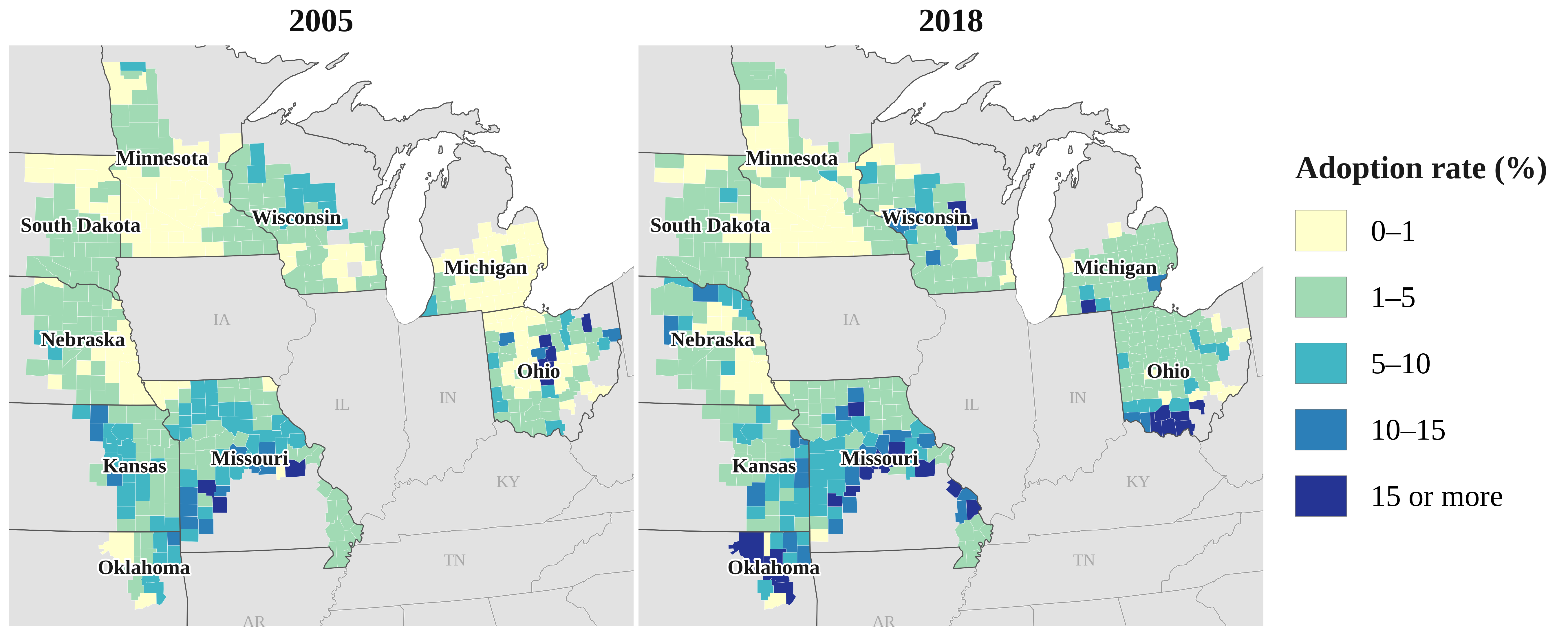
Cover-crop adoption
County patterns, 2005 and 2018.
Key results
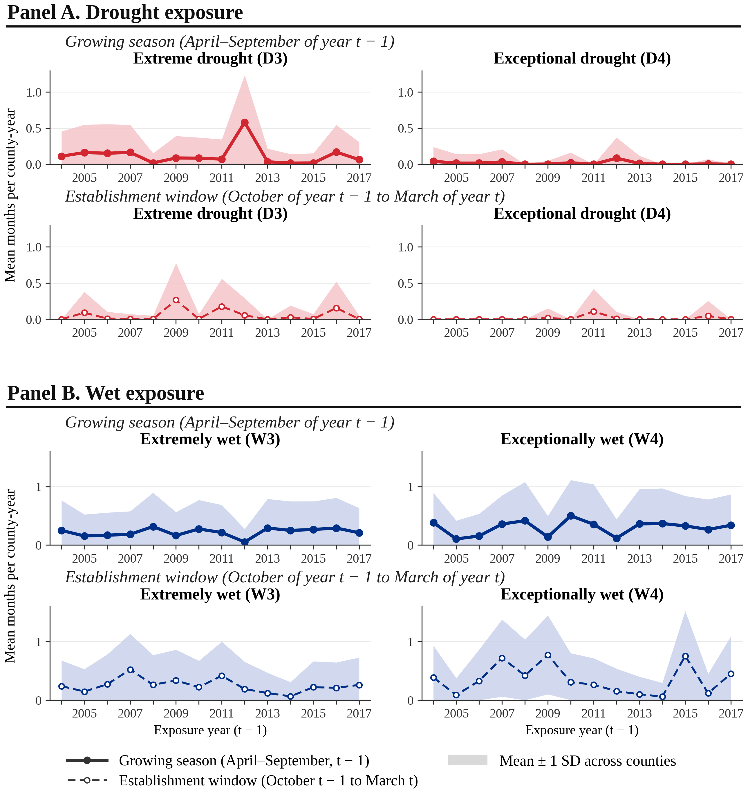
Each additional month of exceptional drought in the preceding growing season was associated with a 1.88-percentage-point decrease in established cover-crop share. Extreme and exceptional wetness were associated with increases of 0.47 and 0.54 percentage points per additional month, respectively.
Baseline estimates, Table 2, Model I; April–September exposure in the preceding year.
Analytical approach
Build the analytical dataset
Combine OpTIS satellite-based cover-crop shares with NOAA/NIDIS moisture indicators and NOAA nClimGrid-Daily weather records in a balanced county-year panel.
Estimate the relationships
Use correlated random-effects fractional logit with county means, year effects, weather controls, and standard errors clustered by county.
Assess timing and robustness
Compare growing-season and establishment exposure, and test alternative weather specifications, lagged exposure, and sensitivity to the 2012 weather year.
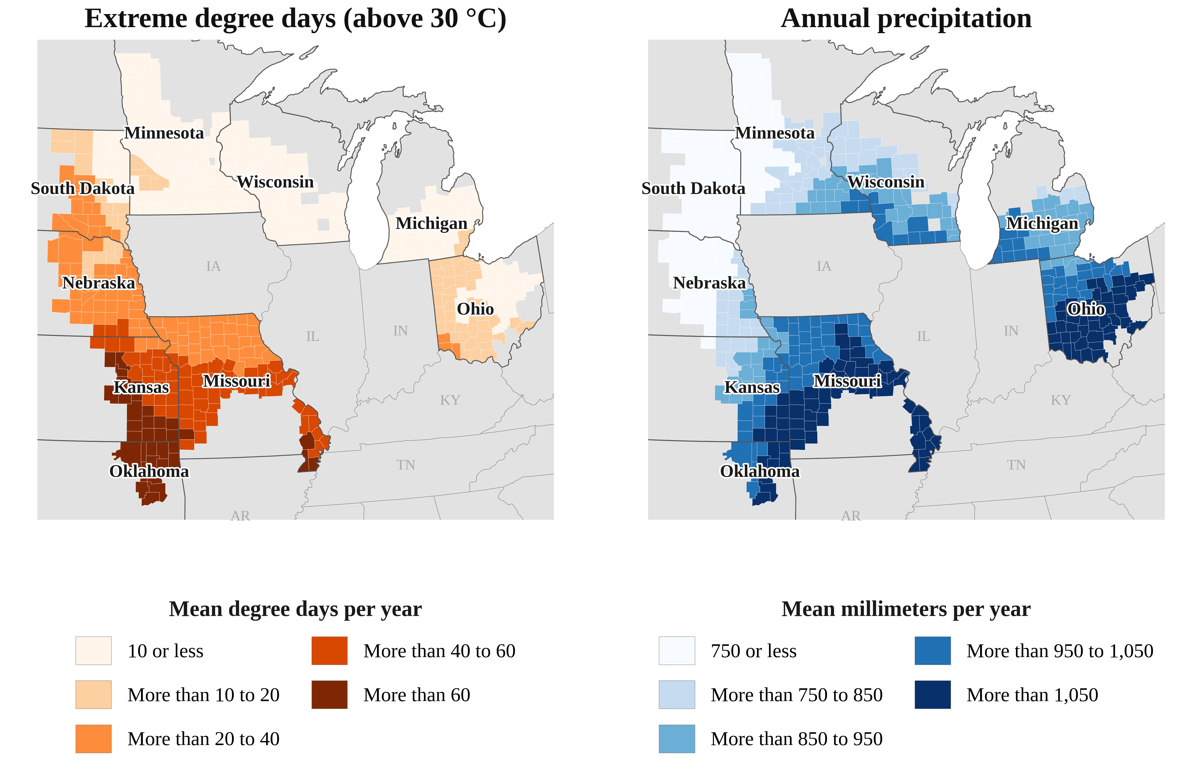
Weather exposure across counties and seasons
Practical relevance
The findings can inform conservation-program timing and technical assistance by identifying weather conditions associated with lower cover-crop establishment.
Interpreting the results
Satellite measures capture established cover crops, so planting intentions cannot be separated from establishment success. The estimates describe county-level associations within the study sample, not causal effects on individual producer decisions.